FCC Broadband Availability
Jaewon R. Choi
The Federal Communication Commission annually publishes raw data collected through the Form 477. With the raw data, the FCC annually publishes Broadband Deployment Report that provides detailed broadband availability at various regional level in percentages of population that could get access to broadband services. However, the ways in which FCC calculates broadband availability from the raw 477 data is not yet clearly known.
Here, we will lay out our own attempt to replicate FCC’s broadband availability calculation and share some preliminary inspection and analysis of the most up-to-date FCC Form 477 data (June, 2019). We thank Dr.Whitecre, Dr.Gallardo, and Mr.Allen Kim at Microsoft for the help they’ve given regarding the calculation process.
Calculating FCC Broadband Availability
Using the raw FCC477 data, we will generate:
pct_bb_fcc_2019: % of broadband availability at the speed of 25/3 per countypct_bb_fcc_50_5_2019: % of broadband availability at the speed of 50/5 per countypct_bb_fcc_100_10_2019: % of broadband availability at the speed of 100/10 per countypct_bb_fcc_250_25_2019: % of broadband availability at the speed of 250/25 per county
#### Import FCC 477 Data of Three States from URL ####

## Write query for three states ME, KS, TX
# Create temporary file space to download the dataset
temp <- tempfile()
temp2 <- tempfile()
# Download dataset for each state, unzip and import to data frame
# Texas as of June 2019
download.file("https://transition.fcc.gov/form477/BroadbandData/Fixed/Jun19/Version%201/TX-Fixed-Jun2019.zip", temp)
unzip(zipfile = temp, exdir = temp2)
fcc477_2019_tx <- read.csv(file.path(temp2, "TX-Fixed-Jun2019-v1.csv"), header = T)
# Kansas as of June 2019
download.file("https://transition.fcc.gov/form477/BroadbandData/Fixed/Jun19/Version%201/KS-Fixed-Jun2019.zip", temp)
unzip(zipfile = temp, exdir = temp2)
fcc477_2019_ks <- read.csv(file.path(temp2, "KS-Fixed-Jun2019-v1.csv"), header = T)
# Maine as of June 2019
download.file("https://transition.fcc.gov/form477/BroadbandData/Fixed/Jun19/Version%201/ME-Fixed-Jun2019.zip", temp)
unzip(zipfile = temp, exdir = temp2)
fcc477_2019_me <- read.csv(file.path(temp2, "ME-Fixed-Jun2019-v1.csv"), header = T)

# Bind into one
fcc477_Jun2019_txksme <- rbind(fcc477_2019_tx, fcc477_2019_ks, fcc477_2019_me)

## Import FCC Staff's block estimates ##
## The dataset provides FCC's estimates of population, households, and housing units per census block ##
## The links are available at https://www.fcc.gov/reports-research/data/staff-block-estimates ##
download.file("https://www.fcc.gov/file/17838/download", temp)
unzip(zipfile = temp, exdir = temp2)
fcc_staff_est_us2018 <- read.csv(file.path(temp2, "us2018.csv"), header = T)

fcc_staff_est_county2018 <- read.csv("https://www.fcc.gov/file/17821/download", header = T)
unlink(temp)
unlink(temp2)
rm(temp)
rm(temp2)

#### Clean Dataset ####
fcc477_Jun2019_txksme <- fcc477_Jun2019_txksme %>%
  mutate(BlockCode = as.character(BlockCode),
         TechCode = as.character(TechCode),
         Consumer = as.character(Consumer)) %>%
  select(Provider_Id, ProviderName, StateAbbr, BlockCode, TechCode, Consumer, MaxAdDown, MaxAdUp) %>%
  mutate(county_fips = str_sub(BlockCode, 1, 5)) %>%
  filter(TechCode != c("60"))

## Staff Estimates for US Census Block Level ##
fcc_staff_est_us2018 <- fcc_staff_est_us2018 %>%
  mutate(block_fips = as.character(block_fips),
         county_fips = str_sub(block_fips, 1, 5)) %>%
  select(stateabbr, county_fips, block_fips, ends_with("2018"))

## County Level Staff Estimates ##
fcc_staff_est_county2018 <- fcc_staff_est_county2018 %>%
  select(Id, Id2, Geography, ends_with("2018")) %>%
  rename(hu2018 = `Housing.Unit.Estimate..as.of.July.1....2018`,
         pop2018 = `Population.Estimate..as.of.July.1....2018`)
The calculation process takes the following general steps:
- Code blocks based on the presence of broadband service at certain speed level
- If the block has the threshold broadband service, the block’s population is considered to have broadband available
- Only keep the blocks that have certain broadband service available
- Aggregate the population numbers at the county level
- Divide the aggregated population (broadband available population) by the total county population estimate provided by the FCC
#### Calculating the Broadband Availability ####
## General process:
## 1. Code blocks based on presence of broadband service at 25/3 Mbps level
## 2. If the block has 25/3 Mbps service the block is considered to have broadband availability
## 3. Aggregate at the county level
## 4. Merge with staff estimates and calculate percentages

### Data as of June 2019 ###
# Step 1 Code blocks based on persence of broadband service (25/3)
fcc477_Jun2019_txksme <- fcc477_Jun2019_txksme %>%
  mutate(broadband_f = as.factor(ifelse(MaxAdDown >= 25 & MaxAdUp >= 3, 1, 0)),
         bb_50_5_f = as.factor(ifelse(MaxAdDown >= 50 & MaxAdUp >= 5, 1, 0)),
         bb_100_10_f = as.factor(ifelse(MaxAdDown >= 100 & MaxAdUp >= 10, 1, 0)),
         bb_250_25_f = as.factor(ifelse(MaxAdDown >= 250 & MaxAdUp >= 25, 1, 0)))
# Join the staff estimates and filter only consumer services
fcc477_Jun2019_txksme <- fcc477_Jun2019_txksme %>%
  left_join(., fcc_staff_est_us2018, by = c("BlockCode" = "block_fips")) %>%
  filter(Consumer == 1)

# Aggregate at the census block level
# Summing the broadband factor variable would let us know if there is a census block with broadband
# availability or not (if there are, the sum would be greater than 0, if there is non, sum would be 0)
fcc477_txksme_block_1 <- fcc477_Jun2019_txksme %>%
  filter(broadband_f == "1") %>%
  distinct(BlockCode, .keep_all = T)
fcc477_txksme_block_2 <- fcc477_Jun2019_txksme %>%
  filter(bb_50_5_f == "1") %>%
  distinct(BlockCode, .keep_all = T)
fcc477_txksme_block_3 <- fcc477_Jun2019_txksme %>%
  filter(bb_100_10_f == "1") %>%
  distinct(BlockCode, .keep_all = T)
fcc477_txksme_block_4 <- fcc477_Jun2019_txksme %>%
  filter(bb_250_25_f == "1") %>%
  distinct(BlockCode, .keep_all = T)

# Aggregate at the county level and merge with FCC staff estimates
fcc477_txksme_county_1 <- fcc477_txksme_block_1 %>%
  group_by(county_fips.x) %>% summarise(pop_bb_county2018 = sum(pop2018)) %>%
  left_join(., fcc_staff_est_county2018, by = c("county_fips.x" = "Id2"))
fcc477_txksme_county_2 <- fcc477_txksme_block_2 %>%
  group_by(county_fips.x) %>% summarise(pop_bb_county2018 = sum(pop2018)) %>%
  left_join(., fcc_staff_est_county2018, by = c("county_fips.x" = "Id2"))
fcc477_txksme_county_3 <- fcc477_txksme_block_3 %>%
  group_by(county_fips.x) %>% summarise(pop_bb_county2018 = sum(pop2018)) %>%
  left_join(., fcc_staff_est_county2018, by = c("county_fips.x" = "Id2"))
fcc477_txksme_county_4 <- fcc477_txksme_block_4 %>%
  group_by(county_fips.x) %>% summarise(pop_bb_county2018 = sum(pop2018)) %>%
  left_join(., fcc_staff_est_county2018, by = c("county_fips.x" = "Id2"))

#### Calculating FCC Deployment Percentages ####
## 477 Data as of June 2019 & Staff Estimates as of 2018 ##
# Calculate broadband percentage by dividing census block population with broadband by total county
# population
fcc477_txksme_county_1 <- fcc477_txksme_county_1 %>%
  mutate(pct_bb_fcc_2019 = pop_bb_county2018 / pop2018)
fcc477_txksme_county_2 <- fcc477_txksme_county_2 %>%
  mutate(pct_bb_fcc_50_5_2019 = pop_bb_county2018 / pop2018)
fcc477_txksme_county_3 <- fcc477_txksme_county_3 %>%
  mutate(pct_bb_fcc_100_10_2019 = pop_bb_county2018 / pop2018)
fcc477_txksme_county_4 <- fcc477_txksme_county_4 %>%
  mutate(pct_bb_fcc_250_25_2019 = pop_bb_county2018 / pop2018)

fcc477_txksme_county_2019 <- fcc477_txksme_county_1 %>%
  left_join(., select(fcc477_txksme_county_2, county_fips.x, pct_bb_fcc_50_5_2019),
            by = c("county_fips.x")) %>%
  left_join(., select(fcc477_txksme_county_3, county_fips.x, pct_bb_fcc_100_10_2019),
            by = c("county_fips.x")) %>%
  left_join(., select(fcc477_txksme_county_4, county_fips.x, pct_bb_fcc_250_25_2019),
            by = c("county_fips.x")) %>%
  select(county_fips.x, pct_bb_fcc_2019, pct_bb_fcc_50_5_2019, pct_bb_fcc_100_10_2019, pct_bb_fcc_250_25_2019)

fcc477_txksme_county_2019[is.na(fcc477_txksme_county_2019)] <- 0
fcc477_txksme_county_2019 <- fcc477_txksme_county_2019 %>%
  mutate(state_fips = str_sub(county_fips.x, 1,2))
Validating the Calculation
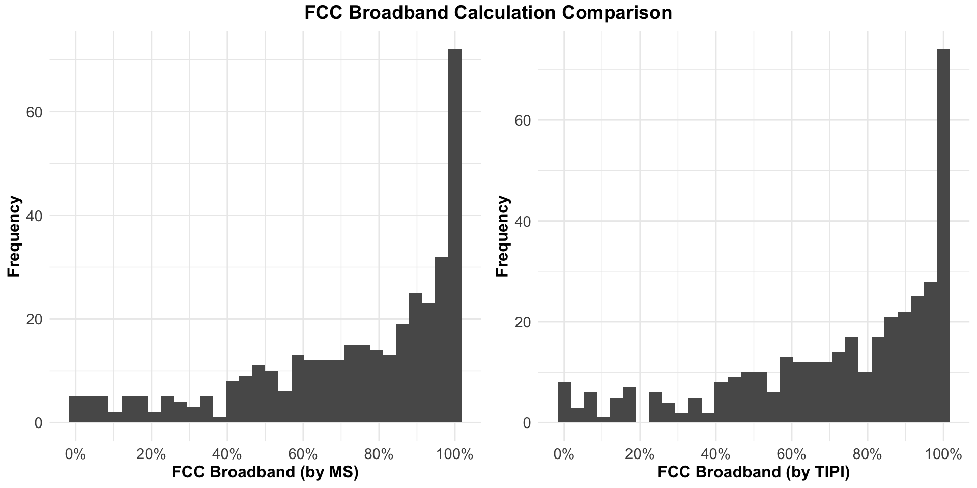
In this section, we will validate our calculation by comparing it to a matching calculation done by Microsoft, which is available here.
## Import 2017 data for time matching ##
### The ending numbers will be cross matched against the numbers in the corresponding FCC deployment report
temp <- tempfile()
temp2 <- tempfile()
# Texas as of Dec 2017
download.file("https://www.fcc.gov/form477/BroadbandData/Fixed/Dec17/Version%203/TX-Fixed-Dec2017.zip", temp)
unzip(zipfile = temp, exdir = temp2)
fcc477_2017_tx <- read.csv(file.path(temp2, "TX-Fixed-Dec2017-v3.csv"), header = T)
# Kansas as of Dec 2017
download.file("https://www.fcc.gov/form477/BroadbandData/Fixed/Dec17/Version%203/KS-Fixed-Dec2017.zip", temp)
unzip(zipfile = temp, exdir = temp2)
fcc477_2017_ks <- read.csv(file.path(temp2, "KS-Fixed-Dec2017-v3.csv"), header = T)
# Maine as of Dec 2017
download.file("https://www.fcc.gov/form477/BroadbandData/Fixed/Dec17/Version%203/ME-Fixed-Dec2017.zip", temp)
unzip(zipfile = temp, exdir = temp2)
fcc477_2017_me <- read.csv(file.path(temp2, "ME-Fixed-Dec2017-v3.csv"), header = T)

unlink(temp)
unlink(temp2)
rm(temp)
rm(temp2)

fcc477_Dec2017_txksme <- rbind(fcc477_2017_tx, fcc477_2017_ks, fcc477_2017_me)

fcc477_Dec2017_txksme <- fcc477_Dec2017_txksme %>%
  mutate(BlockCode = as.character(BlockCode),
         TechCode = as.character(TechCode),
         Consumer = as.character(Consumer)) %>%
  select(Provider_Id, ProviderName, StateAbbr, BlockCode, TechCode, Consumer, MaxAdDown, MaxAdUp) %>%
  mutate(county_fips = str_sub(BlockCode, 1, 5)) %>%
  filter(TechCode != c("60"))

### Data as of Dec 2017 ###
# Step 1 Code blocks based on persence of broadband service (25/3)
fcc477_Dec2017_txksme <- fcc477_Dec2017_txksme %>%
  mutate(broadband_f = as.factor(ifelse(MaxAdDown >= 25 & MaxAdUp >= 3, 1, 0)))
# Join the staff estimates and filter only consumer services
fcc477_Dec2017_txksme <- fcc477_Dec2017_txksme %>%
  left_join(., fcc_staff_est_us2018, by = c("BlockCode" = "block_fips")) %>%
  filter(Consumer == 1)

# Aggregate at the census block level
# Summing the broadband factor variable would let us know if there is a census block with broadband
# availability or not (if there are, the sum would be greater than 0, if there is non, sum would be 0)
fcc477_txksme_block_2017 <- fcc477_Dec2017_txksme %>%
  filter(broadband_f == "1") %>%
  distinct(BlockCode, .keep_all = T)

# Aggregate at the county level and merge with FCC staff estimates
fcc477_txksme_county_2017 <- fcc477_txksme_block_2017 %>%
  group_by(county_fips.x) %>% summarise(pop_bb_county2018 = sum(pop2018))
fcc477_txksme_county_2017 <- fcc477_txksme_county_2017 %>%
  left_join(., fcc_staff_est_county2018, by = c("county_fips.x" = "Id2"))

#### Calculating FCC Deployment Percentages ####
## 477 Data as of June 2019 & Staff Estimates as of 2018 ##
# Calculate broadband percentage by dividing census block population with broadband by total county
# population
fcc477_txksme_county_2017 <- fcc477_txksme_county_2017 %>%
  mutate(bb_pct = pop_bb_county2018 / pop2018)
fcc477_txksme_county_2017 <- fcc477_txksme_county_2017 %>%
  mutate(state_fips = str_sub(county_fips.x, 1,2))
Comparing frequency plots of our FCC availability calculation and Microsoft’s FCC availability calculation, we can see that the distribution of the frequencies resemble each other considerably.
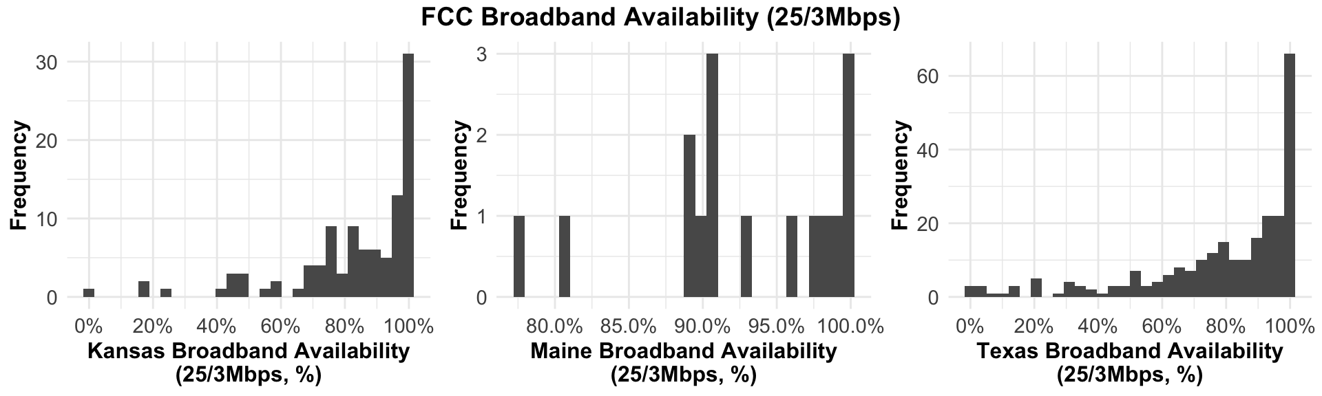
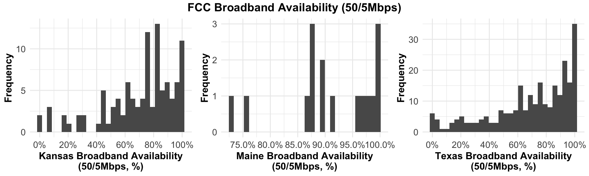
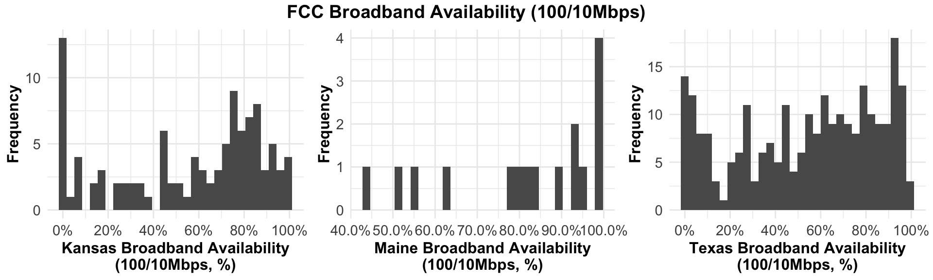
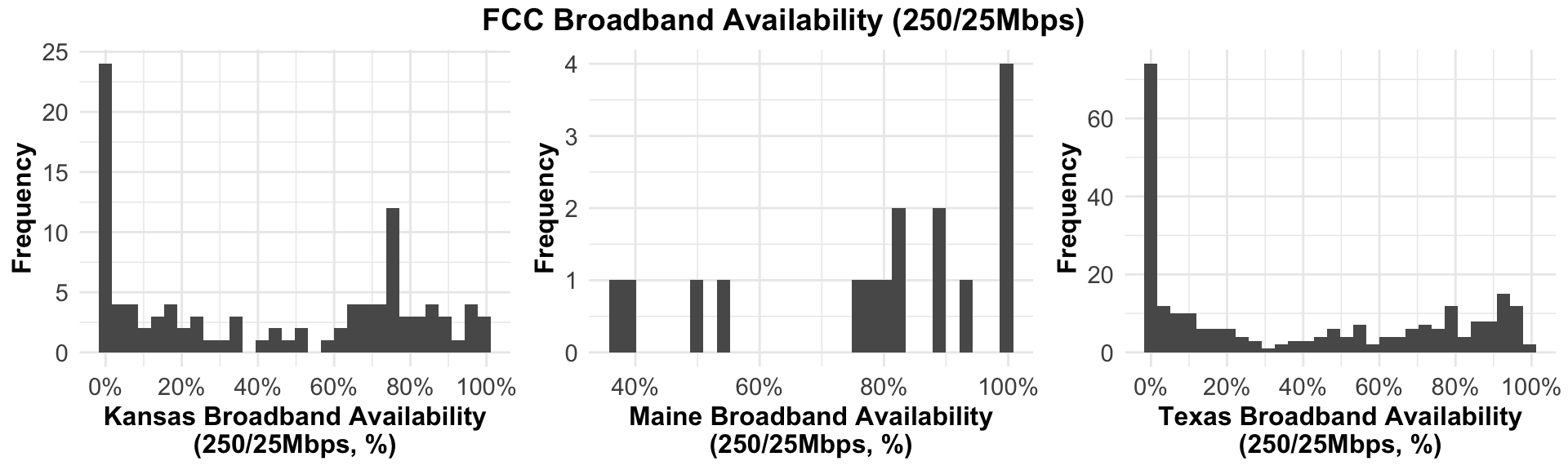
Inspecting FCC Broadband Availability of Texas, Kansas, and Maine
Here we will examine how FCC broadband availaiblity looks like for three different states: Texas, Kansas, and Maine. The following frequency charts are based on the FCC 477 data as of Jun 2019 (v1). In addition to the 25/3 Mbps threshold speed, we will also compare the availability of faster broadband service at the level of 50/5 Mbps, 100/19 Mbps, and 250/25 Mbps.
Copyright © 2020 Jaewon Royce Choi, Technology & Information Policy Institute (TIPI). All rights reserved.